Many simulations are quasi-static, or steady state, because the results are independent of time. Time dependent simulations introduce additional challenges over time independent cases. The data generated during a time dependent simulation could be many gigabytes. Thus, the simulation engineer needs to balance the volume of output data with their needs for data at critical times.
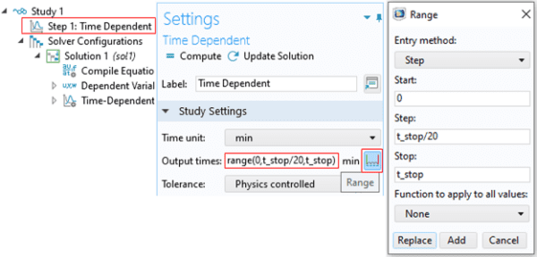
For time dependent simulations, it is important to properly set the output times for storage of the output results. This is usually done by defining the range function range() under the Time Dependent step, as shown in Figure 1.
Figure 1. Standard way to define output times for results storage.
Consider the example where we have a time dependent heat transfer analysis and want to track the average temperature over some domain as a function of time. Let us assume that we have a simple heat source and we expect a smooth monotonic change of temperature over time. In this situation, setting up the required output times is straightforward and we can use a relatively small number of output times.
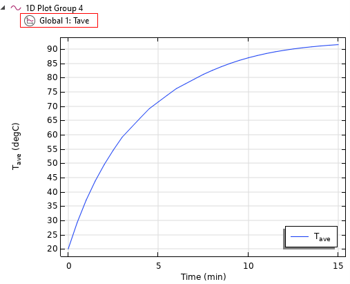
Figure 2 shows an example of the average temperature history. In this case, storing results at a relatively small number of output times (20 points, in our example) is more than enough to adequately characterize the thermal response of the system; the temperature variation is smooth and rises monotonically.
Figure 2. Average temperature history for constant heat source.
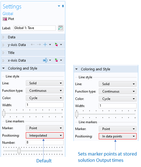
To see the output times of the stored solution, we can activate Line Markers and adjust the setting by choosing the Positioning option ‘In data points’, as shown in Figure 3. This will place line markers exactly at the stored output times specified by the range function.
Figure 3. Options to display line markers.
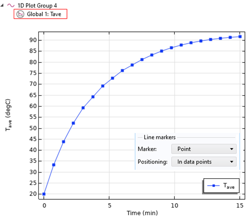
The resulting plot is shown in Figure 4. It is clear that the specified number for stored solutions output times is more than sufficient. In fact, we can even reduce the number of output times to save disk space for the stored model file without losing the key features for the results.
Figure 4. Temperature history with line markers placed at every output time of stored solution.
Simulations with more complex variations in time challenge the simulation engineer to output data at intervals that capture key results. As an example, let us consider a simulation where we want to control the temperature in such a way that the average temperature stays within some limits defined by lower and upper target levels.
The simulation engineer can implement this approach using the Events (ev) interface, as shown in the COMSOL Multiphysics application library, “Modeling the Behavior of a Thermostat”, Application ID: 46781.
The implicit event interface enables us to turn off the heater if the temperature exceeds the upper target limit. When this happens, the thermostat is cooling down. If the temperature falls below the specified lower target level, implicit events interface facilitates switching the state variable and turning on the heat source to increase the temperature. This process of turning the heat source ‘On’ and ‘Off’ is repeated, thus keeping the average temperature within the specified bounds.
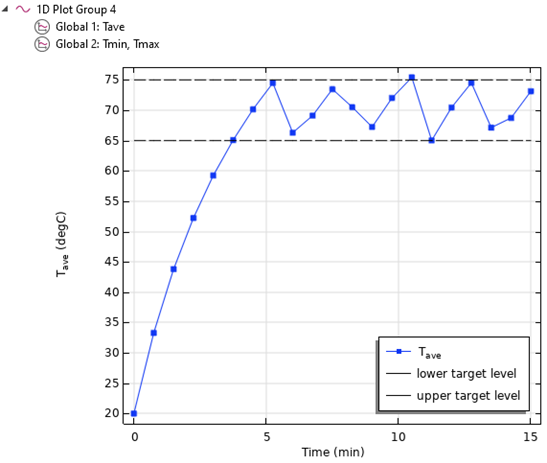
The plot of the average temperature with the Output times setting used so far is shown in Figure 5. The temperature variation shows more complexity than in the previous example, and the sampling frequency is not sufficient to provide adequate resolution of the temperature history. We could refine the range function for output times to store the solution more frequently. However, because heater switching times are not explicitly known, this approach might lead to an excessive amount of data storage required to accurately resolve the sharp variation of temperature when heat source is turned ‘On’ or ‘Off’.
Figure 5. Average temperature with heat source turned ‘On’ or ‘Off’. Stored solutions are controlled by output times.
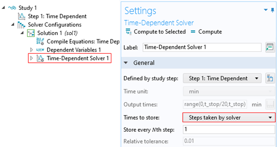
The better way to capture sharp variations in temperature history is to rely on time steps taken by the solver. The solver automatically reduces time stepping to handle high gradients of the dependent variables. The proper way to synchronize output times with solver time stepping is shown in Figure 6. Expand the Solver Configurations node, click Time-Dependent Solver 1 sub-node, then expand the selection General in the Settings window and select Steps taken by solver from the Times to store selection list.
Figure 6. Changing the default control of output times to store solution.
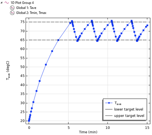
The plot of the temperature history with the adjusted settings to store the solution is shown in Figure 7. This plot shows the features of the temperature variation more accurately than Figure 5 while controlling the volume of data generated.
Figure 7. Average temperature with heat source turned ‘On’ or ‘Off’. Stored solutions are controlled by solver stepping.
This method of controlling data output for time dependent solutions balances the simulation engineer’s desire for sufficient data and limited data file sizes.
We hope you have enjoyed learning about this capability in COMSOL Multiphysics. AltaSim provides these tips from our experience in training engineers how to use COMSOL Multiphysics. Our training focuses on the problem-solving techniques that we have developed using COMSOL Multiphysics to solve our clients’ most challenging simulations.

